This iPython Notebook demonstrates how to generate a map of major Holocene volcanic eruptions. I think it's a good introduction to basic analysis and visualization of georeferenced data with Python tools.
Data is from the Smithsonian Global Volcanism Program. Recently the website was updated with improved search tools and the ability to download database search results to .csv format. I did a global search for eruptions with a volcano explosivity index (VEI) greater than 4. This index is a measure of the magnitude of an explosive volcanic eruption, and can be converted to erupted volume on a logarithmic scale:
| VEI | Description | Plume Height | Volume | Classification | How often | Example |
| 0 | non-explosive | < 100 m | 1000s m3 | Hawaiian | daily | Kilauea |
| 1 | gentle | 100-1000 m | 10,000s m3 | Haw/Strombolian | daily | Stromboli |
| 2 | explosive | 1-5 km | 1,000,000s m3 | Strom/Vulcanian | weekly | Galeras, 1992 |
| 3 | severe | 3-15 km | 10,000,000s m3 | Vulcanian | yearly | Ruiz, 1985 |
| 4 | cataclysmic | 10-25 km | 100,000,000s m3 | Vulc/Plinian | 10's of years | Galunggung, 1982 |
| 5 | paroxysmal | >25 km | 1 km3 | Plinian | 100's of years | St. Helens, 1980 |
| 6 | colossal | >25 km | 10s km3 | Plin/Ultra-Plinian | 100's of years | Krakatau, 1883 |
| 7 | super-colossal | >25 km | 100s km3 | Ultra-Plinian | 1000's of years | Tambora, 1815 |
| 8 | mega-colossal | >25 km | 1,000s km3 | Ultra-Plinian | 10,000's of years | Yellowstone, 2 Ma |
table copied from Oregon State's Volcano World website
We'll use Numpy and Matplotlib for analyzing data and plotting. Load the libraries and make some changes to default plot appearance for starters:
%matplotlib inline
import numpy as np
import matplotlib.pyplot as plt

plt.rcParams['figure.figsize'] = (11.0, 8.5)
fontdict = dict(family='sans-serif',weight='bold',size=16) #NOTE: doesn't effect axes labels
plt.rc('font', **fontdict)
Reading .CSV files with python
An extremely useful utility comes with matplotlib to read csv data into a numpy record array. This automatically converts columns of data to strings, integers, and floats!
from matplotlib.mlab import csv2rec, rec2txt #ported matlab functions
gvp = csv2rec('/Users/scott/Desktop/andes_seminar/GVP_VEI4_Global.csv',skiprows=1)

#print gvp.dtype.fields # uncomment to see all column headers
print 'There are {0} recorded eruptions in this database'.format(gvp.size)
volcanos = np.unique(gvp.volcano_name)
print 'The eruptions have occured at {0} volcanos'.format(volcanos.size)
ind = np.argmax(gvp.start_year)
print 'The most recent eruption was a VEI {0} at {1} in {2}'.format(gvp.vei[ind], gvp.volcano_name[ind], gvp.start_year[ind])
Note that many volcanos have names with strange characters, you can fix them manually this way:
gvp.volcano_name[ind] = 'Eyjafjallajökull' #manual fix
print gvp.volcano_name[ind]
Let's look at a histogram of this data set, binned by eruption size. The colors are set in a list to match the icons we'll use on the map:
fig, ax = plt.subplots()

freq, bins, patches = plt.hist(gvp.vei, bins=np.arange(9),
                                lw=2,
                                alpha=0.5,
                                align='left')
colors = ['k','k','white', 'gray', 'yellow', 'orange', 'red', 'purple']
for p,c in zip(patches, colors): # change bar colors to match map markers
    print p,c
    p.set_facecolor(c)
ax.set_xlabel('VEI')
ax.set_xlim(0,8)
ax.grid()
ax.set_title('Histogram of Large Holocene Eruptions')
plt.savefig('histogram.png', bbox_inches='tight')

Plotting Data on a Map
Matplotlib is a fantastic plotting library, and the Basemap Toolkit is an excellent way to make publication quality maps.
import mpl_toolkits.basemap as bm
import matplotlib.patheffects as PathEffects

# Initialize Global Map
bm.latlon_default = True
fig = plt.figure(figsize=(11, 8.5))
bmap = bm.Basemap(projection='robin',lon_0=0,resolution='c') #Robinson Projection
bmap.drawcoastlines()

That's easy... but boring. Let's add a background. Basemap comes with some built-in background options. For example, shaded relief:
bmap.shadedrelief(scale=0.25)

The default shaded relief background image comes from the Natural Earth website, which has a variety of professional raster images. The "Gray Earth" backdrop is particularly good if you want data to stand out. As long as you have an image with global coverage it's easy to set the background with the warpimage() Basemap method.
background = '/Volumes/OptiHDD/data/natural_earth/medium_res/GRAY_50M_SR_OB/GRAY_50M_SR_OB.jpg'
bmap.warpimage(image=background, scale=0.25)

The scale keyword is used to downsample the resolution by 4x, since we are zoomed out so far. Now we can plot the locations of the eruptions on this background:
def plot_volcanos(volcanos, ms=12, color='r',alpha=0.5):
    ''' draw volcanos on basemap '''
    for i in xrange(volcanos.size):
        v = volcanos[i]
        mark, = bmap.plot(v.longitude, v.latitude, marker='^', ms=ms, mfc=color, mec='white', mew=1, ls='none', alpha=alpha)
    return mark

l = plot_volcanos(gvp)
bmap.warpimage(image=background, scale=0.25)
t = plt.title("Holocene Eruptions VEI > 4")

We can convey more information by coloring and sizing the triangles by the size of the eruption:
def print_info(volcanos):
    print 'Name, Eruption Year, Tephra Volume'
    for i in xrange(volcanos.size):
        v = volcanos[i]
        textstr = v.volcano_name + ', ' + str(v.start_year) + ', ' + str(v.tephra_volume)
        print textstr
vei4 = (gvp.vei == 4) # Pelee 1902, Eyjafjallaiokull 2010
vei5 = (gvp.vei == 5) # St Helens 1980m Vesuvius 79
vei6 = (gvp.vei == 6) # Pinatubo 1991, Krakatoa 1883, Huaynaputina 1600
vei7 = (gvp.vei == 7) # Tambora 1815, Mazama 5600B.C.
vei8 = (gvp.vei == 8) # Yellowstone 640,000 BC, Toba 74,000 BC, Taupo 24,500 BC
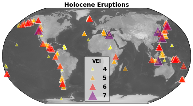
plt.title('Holocene Eruptions')
bmap.warpimage(image=background, scale=0.25)
v4 = plot_volcanos(gvp[vei4],10,'yellow')
v5 = plot_volcanos(gvp[vei5],16,'orange')
v6 = plot_volcanos(gvp[vei6],22,'red')
v7 = plot_volcanos(gvp[vei7],30,'purple')
plt.legend( [v4,v5,v6,v7], ['4','5','6','7'],
numpoints=1,
loc='lower center',
title='VEI',
framealpha=0.7,
shadow=True)
plt.savefig('map.png', bbox_inches='tight')
print_info(gvp[vei7]) # print info on the largest eruptions

Notice that eruptions concentrate on active plate boundaries. Despite having many of the world's active volcanos, the Andes Cordillera on the western margin of South America has no documented Holocene eruption of VEI>6. What was the largest eruption in the Andes?
SA = gvp[gvp.region == 'South America']
biggest = (SA.vei == 6)
print_info(SA[biggest])
Turns out it was Huaynaputina Volcano in Peru in 1600. You can check out Huaynaputina's page on the Smithsonian website here Let's see what else we can find out about Huaynaputina from this database:
def pprint_records(recarray):
    for key in recarray.dtype.names:
        #print '{0}:\t\t {0}'.format(key, recarray[key])
        print '{0:25}{1}'.format(key, recarray[key]) #fix first entry to 25 spaces
huayna = SA[SA.volcano_name == 'Huaynaputina']
pprint_records(huayna)
That's it for now! The iPython notebook is a great way to interactively explore data sets and simultaneously keep a copy of your work. If you wanted to share the notebook as a regular python script, or pdf (requires LaTeX) you can do that too pretty easily with the following ipython terminal commands:
ipython nbconvert --to python mapping_volcanic_eruptions.ipynb
ipython nbconvert --to latex --template article --post PDF mapping_volcanic_eruptions.ipynb